This article was originally published on Medium:
https://medium.com/vertices-and-faces/practical-applications-of-the-dot-product-c5503c2e454e
I recently started at Standard Cyborg where I've been ramping up on Computational Geometry. I've started diving into our lower level source code to see how it ticks. This post documents my learnings about the dot product.
What we'll cover
- Projecting a vector onto a vector
- Finding the orthogonal component of a vector to another vector
- Finding the shortest distance from a point to a segment
Projecting a vector onto a vector
Projecting a vector is one of the simpler practical things we can do with a dot product
Below is a proof explaining how the demo works. After that is a few shorter related demos and proofs.
Math notation refresher
As a courtesy to those who haven't touched Math in a while, here's some notation Linear Algebra notation we'll be using:

"^" (aka hat) is known as the unit vector
Proof
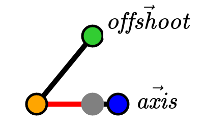
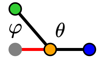
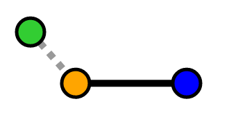
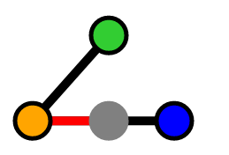
Let the "orange" to "blue" vertices be our axis vector and "orange" to "green" be our offshoot vector. This is the largest proof so we'll take it on in 3 steps.
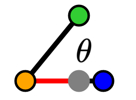
Step 1: Resolving cosine
We have an angle θ between our 2 vectors. This angle has 3 scenarios (assuming -π ≤ θ ≤ π):
-π/2 < θ < π/2
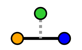
θ = -π/2, θ = π/2
-π ≤ θ < -π/2, π/2 < θ ≤ π
In our first scenario (-π/2 ≤ θ < π/2), we first focus on 0 ≤ θ < π/2. For the sake of brevity, I'm going to handwave over the existence of a right triangle with our projection vector. Please see the gists at the end for a robust proof.
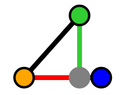
Visualization of our right triangle
By the cosine trigonometric identity, we have:
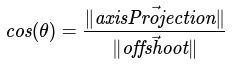
For -π/2 < θ < 0, we build a similar triangle and yield the same cos(θ) equation.
For our second scenario (θ = -π/2, θ = π/2), our offshoot vector is orthogonal and thus our projection vector is the zero vector. We can still use the same cos(θ) equation.
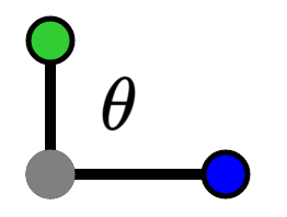
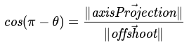
For our third scenario (-π ≤ θ < -π/2, π/2 < θ ≤ π), we will focus on π/2 < θ ≤ π. We build a right triangle similar to above but ours is with φ:
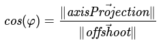
Cosine trigonometric identity for right triangles

Definition of supplementary angles
Substitution of φ
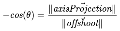
Equivalence via cosine identities
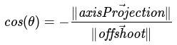
Multiplication by -1
For our -π ≤ θ < -π/2 case, we build a similar triangle and yield the same cos(θ) equation.
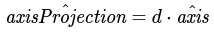
Now that we've resolve cosine for each of our scenarios, we can consolidate them. If cos(θ) ≥ 0, then let d = 1. Otherwise, let d = -1. This allows us to restate:
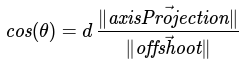
New cosine definition with direction
Additionally, we can define our projection unit vector using d:
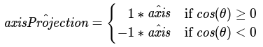
Piece-wise axis projection unit vector definition
Direction based axis projection unit vector definition
Step 2: Restructure dot product
To make our final derivation easier, we're going to restructure the dot product a little. First, let's start by writing out more knowns:
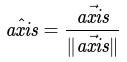

Definition of unit vectors
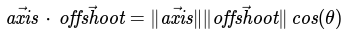
Dot product derivation from http://heaveninthebackyard.blogspot.com/2011/12/derivation-of-dot-product-formula.html
With these knowns, we restructure our axis projection vector as follows:
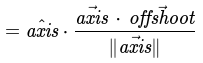
Taken from knowns above
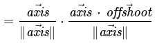
Substitute cosine with equation from previous step
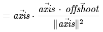
Cancel out fractions
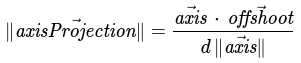
Divide both sides by direction and axis vector length
Step 3: Calculate projection vector
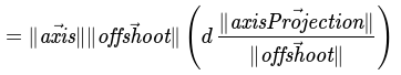
Taken from knowns above
Substitute unit vectors and axis projection length from previous steps
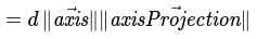
Cancel out directions
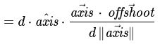
Substitute unit vector definition
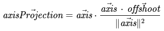
Simplify formula to vector times a scalar
And there we go, we have our formula for a projection vector:
Finding the orthogonal component of a vector to another vector
With the calculation above, we can derive an orthogonal component of a vector with respect to another vector
This is practical for computing an angle between 2 vectors around a given axis in 3 dimensional space (e.g. rotation around a fixed axis).
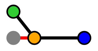
For the proof, we've already resolved this vector via our right triangle construction; it's the "opposite" edge (i.e. our green line). As a result, we can use vector addition to resolve our orthogonal vector:

Construction of our vector via its right triangle

Subtraction and rearrangement of vectors
For some sanity, we can also think of our vector space with our axis as an actual axis:
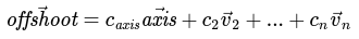
Definition of offshoot in terms of vectors

Definition of axisProjection in terms of vectors

Subtraction of our definitions and proof of orthogonality
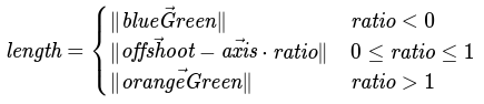
Finding the shortest distance from a point to a segment
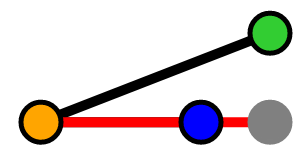
For this proof, we will solve it in a piece-wise fashion. There are 3 scenarios:
Our point is "behind" our segment
Our point is "between" our segment

Our point is "ahead of" our segment
In the "behind" and "ahead of" scenarios, the shortest distance will be to the closest vertex. In the "between" scenario, the shortest distance will be a perpendicular line from the segment to the point.
To determine which of these scenarios our point falls into, we find the projection vector and compare it to our segment as a vector. We simplify this a little so it's a comparison between their scalars, not their vectors
Equations:
Previous resolution from "Projecting a vector onto a vector"
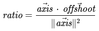
Ratio between axis projection and axis vectors
This ratio tells us how much of our offshoot vector is projecting onto our axis.
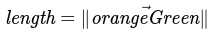
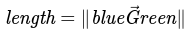
If the ratio is negative, then we know the point is "behind" our segment and our length is the distance from our "orange" point to "green" point:
Otherwise if the ratio is greater than 1, then we know our projection vector is longer than the axis vector itself. Thus, the point is "ahead" of our segment and our length is the distance from our "blue" point to our "green" point:
Otherwise, the ratio is between 0 and 1 inclusively, so our projection vector falls onto the segment. Thus, the shortest distance is a line perpendicular to the line. We've calculated this before via the orthogonal component of a vector:
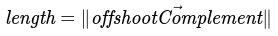
Ideal length definition
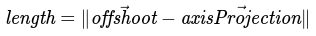
Vector addition expansion
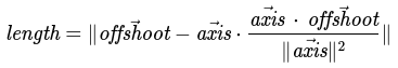
Substitution for axis projection calculation
We can shorten this a little bit with some variable reuse:
Substitution for ratio calculated above
Here's our final solution in a piece-wise format: